Coloring the galaxy
or: How I spend my weekends
How does one take a picture of the Milky Way? With good technique and the right equipment you can do so with a camera, an opportunity I try not to miss when vacationing under the dark skies of the American West (see photo). But stray light and sensor noise limit the dynamic range achievable with this technique. Is there another approach? Well, if we knew where all the stars in the night sky were, we could render their light with any brightness, field-of-view, or PSF we wished. And thanks to the Two Micron All-Sky Survey (2MASS), we have precisely the data we need.
Unfortunately, the dataset is formidable in size, and it’s not obvious how to to extract the information we want. In particular, how bright is each star, and what color are they? I was curious about these questions recently, so here is the approach I took to answer them. The resulting source code is available in my TooMassFun repository on GitHub.
Having acquired the 40 GB (compressed) dataset (hooray for university Internet), there are immediately two questions we need to answer:
- Which fields are relevant to our solution?
- How can we extract those fields from the provided data?
The PSC fields are documented on the 2MASS website. To make an image, we need to know three things: position, brightness, and color. Position is straightforward – the “ra” and “dec” fields are basically longitude and latitude for the sky. They are measured in degrees: 0°–360° and -90°–90°. Brightness and color are less obvious, though. The stars in this catalog have been measured in three near-IR filters (J,H,Ks), and the measured flux in each band has been converted to a magnitude. One approach would be to choose one of the bands as a proxy for visible brightness, but this is ad-hoc and wouldn’t give any indication of color. Instead, we will assume that stars are black-body radiators, fit a Planck distribution to these fluxes, and derive both color and brightness from this distribution. The details will come later; what’s important is that these three magnitudes are sufficient for the job.
Now that know which fields we need (columns 1, 2, 7, 11, & 15, along with 9, 13, and 17 to take advantage of uncertainties when fitting), how do we extract them? The columns are delimited by pipes (‘|’), and the data is gzip compressed. I chose to use Scala for the parser here (see PscConvert), since it makes it easy to read gzipped data, split lines of text on delimiters, convert strings to numbers, and perform tasks in parallel (there are 92 files, after all). Furthermore, I just like the language. What comes next? Well, here’s where things get technical.
A lot can happen to a photon between a star and a detector. It could be scattered by the ISM, absorbed by the atmosphere, deflected by the telescope, or just fail to interact with the sensor. Thankfully, the survey team has derived calibrations to account for most of these effects. Using the parameters in the 2MASS explanatory supplement, along with the definition of “magnitude” (an incredibly frustrating unit), we can convert filter magnitudes to integrated energy fluxes and propagate their uncertainties as well. These fluxes correspond to photons hitting the top of the Earth’s atmosphere that lie within an effective bandpass for each filter. In other words, we can now characterize some small portions of each star’s spectrum as it would be observed by a satellite orbiting the Earth.
Now our assumption that stars are black-body radiators is a pretty good one, but by the time the photons have reached Earth, their interactions with the ISM mean that their spectrum is no longer guaranteed to be Planckian. For the purposes of this project, however, we neglect this effect. The spectrum’s deviation from a black-body form is probably small (especially given our artistic purpose), and correcting for it would take us beyond the scope of this dataset.
So our goal is now to fit a Planck distribution to these three measurements. Such a distribution is described by only two parameters: a “temperature”, and an overall amplitude scale. Since the function is linear in the amplitude, this reduces to a 1D minimization problem for the residual as a function of temperature. I chose to implement this procedure in C using routines from GSL (see mags2temp).
Once we have the parameters of each star’s spectral distributions, computing their colors and brightnesses is formally straightforward. Working in CIE XYZ space, we simply integrate each star’s distribution against three different color matching functions, available from CVRL. From there, converting to sRGB for display on a computer is simply a matter of looking up the conversion formulas. But for the moment, we’ll stick to CIE XYZ for one simple reason: it’s linear. In other words, to compute the color resulting from seeing two stars at once, you simply add their color coordinates (this is NOT true of gamma-corrected color spaces like sRGB).
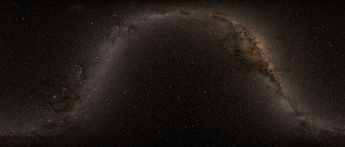
Now that we know the brightness and color of each star, along with their positions, it’s time to generate an image. This is a perfect job for GPUs! I chose to implement the following procedures in C++ and CUDA (see SkyRender), making use of the OpenCV library (which I learned to use in Udacity’s CS344 course). Most of the remaining operations are pretty simple: figure out the pixel location of each star from its sky coordinates (many projections are possible, but we’ll keep things simple and cylindrical), add the colors from all stars at each pixel, truncate to an overall brightness scale, and convert to sRGB. But there’s one thing missing: when starlight hits any optical system, whether a telescope or the human eye, its light spreads out over the detector according to a “point spread function.” Mathematically, this is a convolution with some instrument-specific kernel. For our purposes, we could compute the kernel for some idealized telescope (which would take the form of an Airy disk), or we could invent our own kernel optimized for aesthetics. Some colleagues of mine found “exp(-sqrt(r/w))” to work well, where “r” is the distance in pixels from the center of the star and “w” is a characteristic width, chosen to taste.
Combining all these pieces gives us the image above. Thus, with a mix of statistics, physics, color theory, and programming, along with a great open dataset, we can create beautiful renderings of the night sky without ever having to freeze our fingers off outdoors. I hope you enjoyed this little problem-solving adventure; you now have a pretty good idea of how graduate students spend their weekends ☺.
[authoring in-progress; additional figures pending]
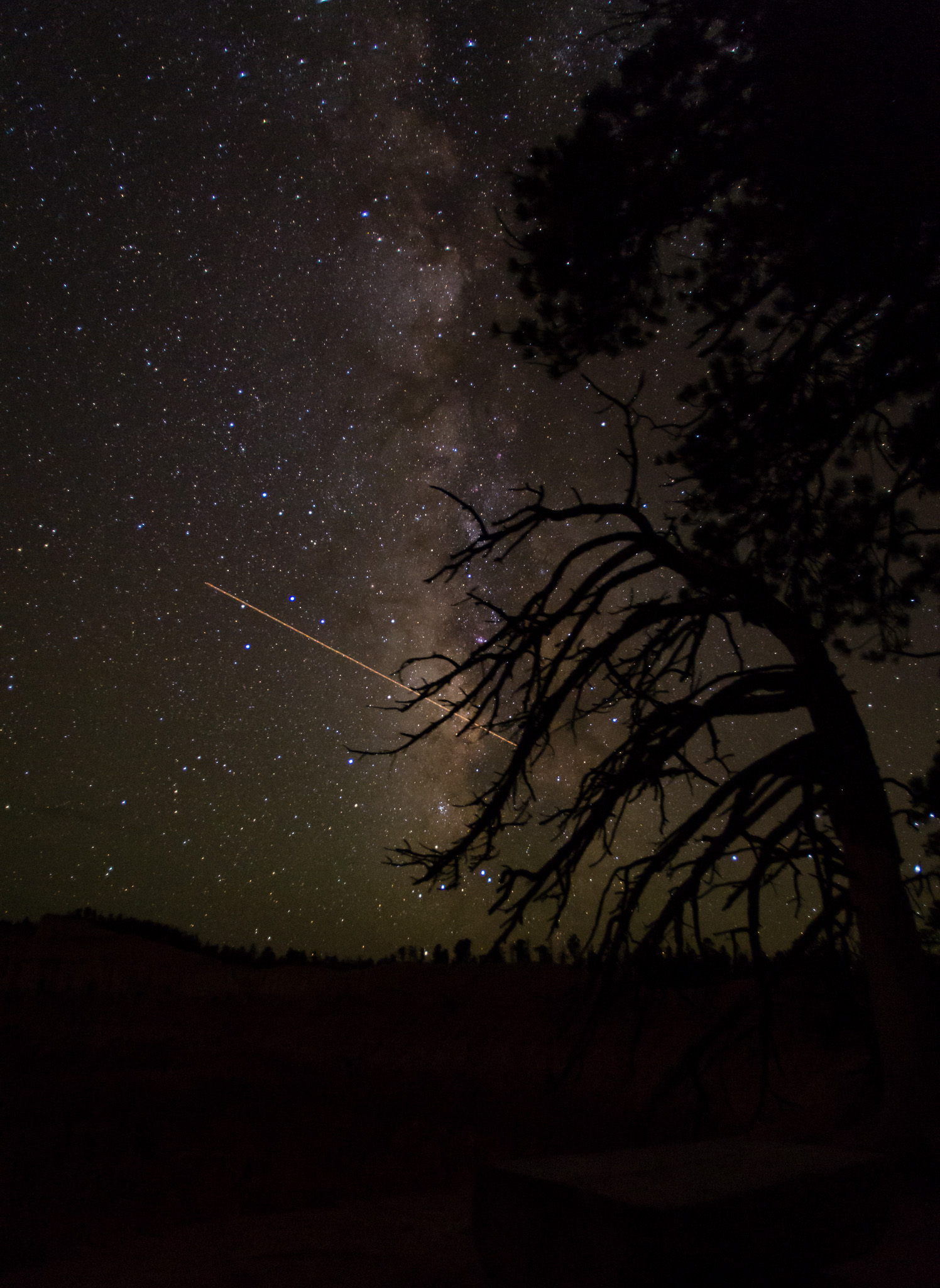
Milky Way over Bryce Canyon, 28 August 2013